Working with Categorical Hyperparameters
categorical-hyperparameters.Rmd
library(spacefinder)
library(data.table)
library(ggplot2)
data(benchmark_data)
Introduction
Many hyperparameter optimization scenarios involve categorical
hyperparameters like optimizer type, activation function, or kernel
choice. The spacefinder package handles these by fitting
separate subspaces for each categorical level.
The Data
The benchmark_data includes three optimizers: SGD, Adam,
and RMSprop. Let’s explore how they differ:
# Performance by optimizer
benchmark_data[, .(
  mean_auc = mean(auc),
  median_auc = median(auc),
  sd_auc = sd(auc),
  max_auc = max(auc),
  n = .N
), by = optimizer]
#>    optimizer  mean_auc median_auc     sd_auc max_auc     n
#>       <char>     <num>      <num>      <num>   <num> <int>
#> 1:       SGD 0.8346208  0.8554099 0.11751028       1  2500
#> 2:      Adam 0.6010436  0.5762377 0.09207576       1  2500
#> 3:   RMSprop 0.6884296  0.6504798 0.14778183       1  2500

# Visualize distributions
ggplot(benchmark_data, aes(x = auc, fill = optimizer)) +
  geom_density(alpha = 0.6) +
  theme_minimal() +
  labs(title = "AUC Distribution by Optimizer",
       x = "AUC", y = "Density") +
  theme(legend.position = "top")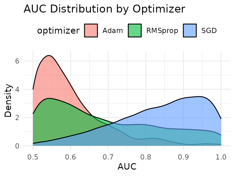
Notice that Adam tends to achieve slightly higher performance than SGD and RMSprop.
Creating a Task with Categorical Hyperparameters
Include the categorical hyperparameter in the task definition:
# Explicit specification
task <- TaskSubspace$new(
  data = benchmark_data,
  target_measure = "auc",
  hps = c("learning_rate", "max_depth"),
  cat_hps = "optimizer"
)

# Formula interface and convenience function
task <- as_task_subspace(
  data = benchmark_data,
  formula = auc ~ (learning_rate + max_depth) * optimizer
)
The * optimizer in the formula indicates that separate
subspaces should be fitted for each optimizer type.
Fitting Separate Subspaces
Train a learner - it will automatically fit one subspace per optimizer:
learner <- LearnerSubspaceBox$new(task)
learner$train(q_val = 0.9)
Examining Results per Category
Coefficients
The coefficients now show separate bounds for each optimizer:
bounds <- coef(learner)
print(bounds)
#>    optimizer hyperparameter          min         max
#>       <char>         <char>        <num>       <num>
#> 1:       SGD  learning_rate 0.0000646238  0.06077546
#> 2:       SGD      max_depth 3.0000000000 15.00000000
#> 3:      Adam  learning_rate 0.0008549492  0.01177603
#> 4:      Adam      max_depth 7.0000000000 11.00000000
#> 5:   RMSprop  learning_rate 0.0001591802  0.07528367
#> 6:   RMSprop      max_depth 4.0000000000 14.00000000
Notice how different optimizers have different optimal ranges!
# Compare learning rate ranges
bounds[hyperparameter == "learning_rate"] |>
  ggplot(aes(optimizer, color = optimizer)) +
  geom_errorbar(aes(ymin = min, ymax = max), width = 0.2, linewidth = 1) +
  scale_y_log10() +
  theme_minimal() +
  labs(title = "Optimal Learning Rate Range by Optimizer",
       y = "Learning Rate (log scale)", x = "Optimizer") +
  theme(legend.position = "none")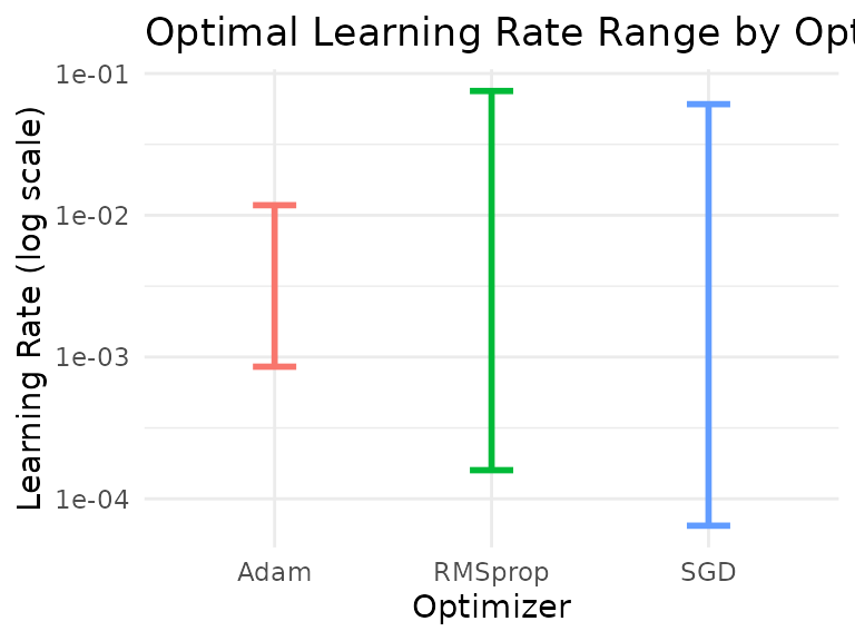
Summary
The summary shows fitting statistics for each optimizer:
summary(learner)
#> SUMMARY
#> --------------------------------------------------
#> Property                      Value
#> ----------------------------  -------------------------
#> Target Measure                auc
#> Numeric Hyperparameters       learning_rate, max_depth
#> Categorical Hyperparameters   optimizer
#>
#>
#> COEFFICIENTS
#> --------------------------------------------------
#> optimizer   hyperparameter          min          max
#> ----------  ---------------  ----------  -----------
#> SGD         learning_rate     0.0000646    0.0607755
#> SGD         max_depth         3.0000000   15.0000000
#> Adam        learning_rate     0.0008549    0.0117760
#> Adam        max_depth         7.0000000   11.0000000
#> RMSprop     learning_rate     0.0001592    0.0752837
#> RMSprop     max_depth         4.0000000   14.0000000
#>
#>
#> STATUS
#> --------------------------------------------------
#> optimizer   status    objective_value   n_violations   observations
#> ----------  -------  ----------------  -------------  -------------
#> SGD         NULL                 NULL           NULL            250
#> Adam        NULL                 NULL           NULL            250
#> RMSprop     NULL                 NULL           NULL            250
Each optimizer gets its own row in the status table, showing: - Number of observations used - Performance across tasks
Visualization
The autoplot function creates separate visualizations for each optimizer:
lapply(autoplot(learner), \(plot) plot + scale_x_continuous(limits = c(0, .01)))
#> $SGD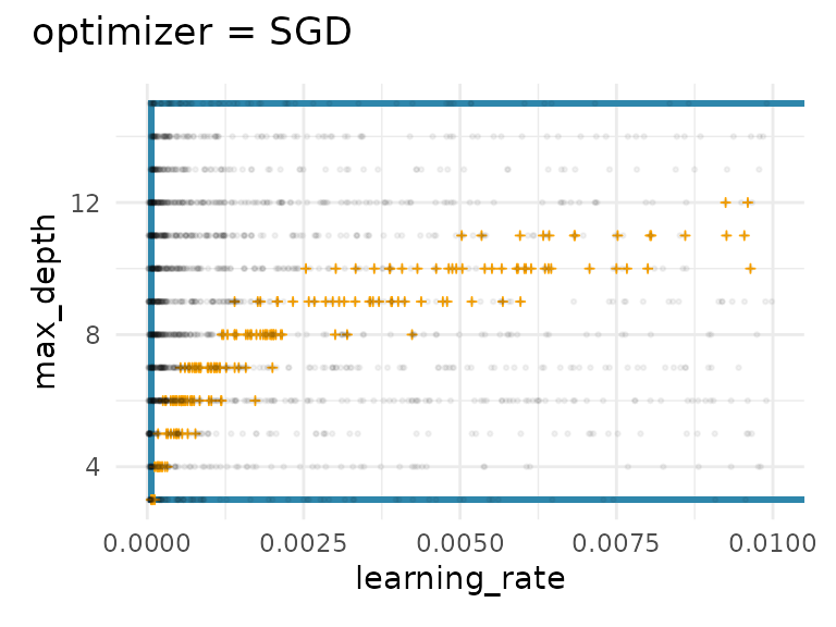
#>
#> $Adam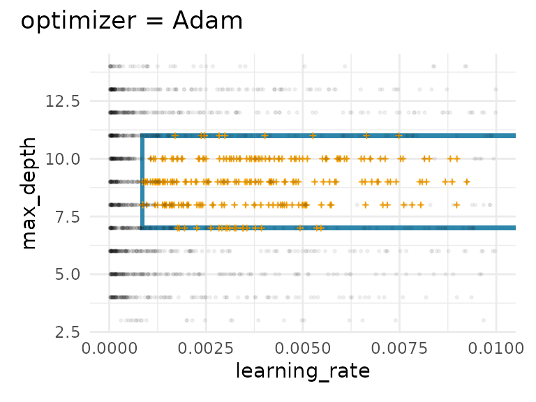
#>
#> $RMSprop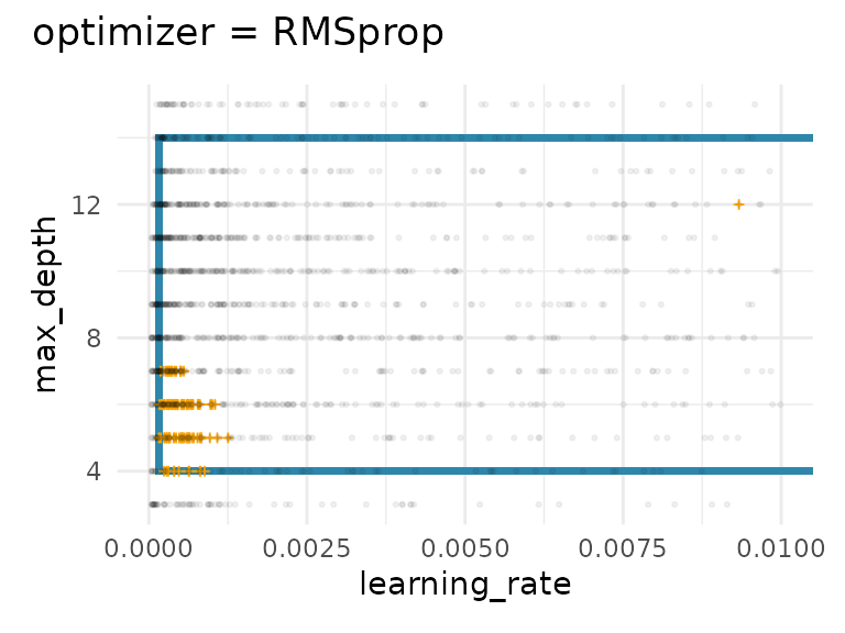
Each panel shows: - The fitted subspace for that optimizer - Top configurations for that optimizer (orange crosses) - All configurations for that optimizer (gray points)
Comparing Optimizers
Let’s analyze the differences between optimizers:
# Extract top configs per optimizer
top_configs_summary <- learner$top_configs[, .(
  mean_lr = mean(learning_rate),
  median_lr = median(learning_rate),
  mean_depth = mean(max_depth),
  median_depth = median(max_depth),
  mean_auc = mean(auc),
  n = .N
), by = optimizer]

print(top_configs_summary)
#>    optimizer     mean_lr   median_lr mean_depth median_depth  mean_auc     n
#>       <char>       <num>       <num>      <num>        <num>     <num> <int>
#> 1:       SGD 0.008340861 0.003586301      8.972            9 0.9888067   250
#> 2:      Adam 0.003784583 0.003486343      8.952            9 0.8105505   250
#> 3:   RMSprop 0.015224210 0.012173355      9.204           11 0.9642822   250
# Scatter plot colored by optimizer
ggplot(learner$top_configs, aes(x = learning_rate, y = max_depth,
                                 color = optimizer, shape = optimizer)) +
  geom_point(size = 2, alpha = 0.7) +
  scale_x_log10() +
  theme_minimal() +
  labs(title = "Top Configurations by Optimizer",
       x = "Learning Rate (log scale)", y = "Max Depth") +
  theme(legend.position = "top")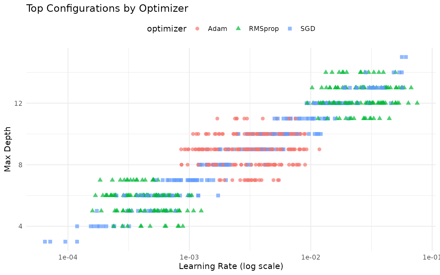
Next Steps
-
vignette("learner-comparison"): Compare Box, Polygon, and Ellipsoid learners -
vignette("density-estimation"): Add probabilistic density withaugment()
sessionInfo()
#> R version 4.5.2 (2025-10-31)
#> Platform: x86_64-pc-linux-gnu
#> Running under: Ubuntu 24.04.3 LTS
#>
#> Matrix products: default
#> BLAS:   /usr/lib/x86_64-linux-gnu/openblas-pthread/libblas.so.3
#> LAPACK: /usr/lib/x86_64-linux-gnu/openblas-pthread/libopenblasp-r0.3.26.so;  LAPACK version 3.12.0
#>
#> locale:
#>  [1] LC_CTYPE=C.UTF-8       LC_NUMERIC=C           LC_TIME=C.UTF-8
#>  [4] LC_COLLATE=C.UTF-8     LC_MONETARY=C.UTF-8    LC_MESSAGES=C.UTF-8
#>  [7] LC_PAPER=C.UTF-8       LC_NAME=C              LC_ADDRESS=C
#> [10] LC_TELEPHONE=C         LC_MEASUREMENT=C.UTF-8 LC_IDENTIFICATION=C
#>
#> time zone: UTC
#> tzcode source: system (glibc)
#>
#> attached base packages:
#> [1] stats     graphics  grDevices utils     datasets  methods   base
#>
#> other attached packages:
#> [1] ggplot2_4.0.1          data.table_1.18.0      spacefinder_0.2.2.0000
#>
#> loaded via a namespace (and not attached):
#>  [1] Matrix_1.7-4       bit_4.6.0          gtable_0.3.6       jsonlite_2.0.0
#>  [5] Rmpfr_1.1-2        compiler_4.5.2     Rcpp_1.1.0         jquerylib_0.1.4
#>  [9] systemfonts_1.3.1  scales_1.4.0       textshaping_1.0.4  yaml_2.3.12
#> [13] fastmap_1.2.0      lattice_0.22-7     R6_2.6.1           patchwork_1.3.2
#> [17] labeling_0.4.3     generics_0.1.4     knitr_1.51         backports_1.5.0
#> [21] checkmate_2.3.3    desc_1.4.3         bslib_0.9.0        RColorBrewer_1.1-3
#> [25] rlang_1.1.6        cachem_1.1.0       CVXR_1.0-15        xfun_0.55
#> [29] S7_0.2.1           fs_1.6.6           sass_0.4.10        bit64_4.6.0-1
#> [33] cli_3.6.5          withr_3.0.2        pkgdown_2.2.0      digest_0.6.39
#> [37] grid_4.5.2         gmp_0.7-5          lifecycle_1.0.4    vctrs_0.6.5
#> [41] evaluate_1.0.5     glue_1.8.0         farver_2.1.2       ragg_1.5.0
#> [45] rmarkdown_2.30     tools_4.5.2        htmltools_0.5.9